bayesian skyline plot tutorial

bayesian skyline plot tutorial

brendonfrieling55125    March 31, 2022    Comment   

In the field of anthropological genetics for example implementing Bayesian skyline plots and approximate Bayesian computation is becoming ubiquitous as means to analyze genetic data for the purpose of demographic or historic inference. Second half of tutorial found at.

Skyline Plots

Bayesplot is an R package providing an extensive library of plotting functions for use after fitting Bayesian models typically with MCMC.

. Perhaps the most popular demographic model in use today is the Bayesian skyline plot BSP which allows the effective population size to change in a piecewise fashion at coalescent events Ho and Shapiro 2011. Here we present the Extended Bayesian Skyline Plot a non-parametric. The main di erence is in the de-mographic model which is a linear piecewise model instead of constant piece-wise model.

Tutorials There are some general notes that apply to all tutorials. Coalescent Bayesian Skyline analysis output. In this tutorial we will estimate the dynamics of the Egyptian Hepatitis C epidemic from genetic sequence data collected in 1993.

Bayesian skyline plots for each lineage showed three features Fig. The so-called Skyline methods allow to extract this information from phylogenetic trees in a. These tutorials use the graphical applications of BEAST to perform analyses using the provided example files.

Effective population size N e is related to genetic variability and is a basic parameter in many models of population genetics. Dedicated analytical methods including Bayesian skyline plots BSPs and approximate Bayesian computation ABC. STAR BEAST Version 203.

The aim of this tutorial is to. 2000 and generalized skyline plots Strimmer and Pybus 2001 estimate changes in. Below the mcmc block is provided of the BEAST XML example for a Bayesian skyline plot model BSP and an uncorrelated relaxed clock model with an underlying lognormal distribution UCLD.

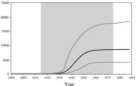
The publication is accompanied by 2 example BEAST XML files to indicate how to use the different estimators in BEAST which is also what this tutorial focuses on. Select the Coalescent Extended Bayesian Skyline model for each locus we unlinked all of the trees in the Partitions panel. The two blue lines are the upperandlowerboundsofthe95HPDinterval.

The predecessors to the BSP the classic Pybus et al. In the field of anthropological genetics for example implementing Bayesian skyline plots and approximate Bayesian computation is becoming ubiquitous as means to analyze genetic data for the purpose of demographic or historic inference. The plots created by bayesplot are ggplot objects which means that after a plot is created it can be further customized using various functions from the ggplot2 package.

Second a relatively flat ancient demography appeared in the BSPs for each lineage and was followed by an apparent increase in the distant past in lineages A and C. Correspondingly there is a critical need for better understanding of the underlying assumptions proper. The coalescent ex-plores the history of a population by creating a gene genealogy or genealogical tree representing the.

A previous analysis of Pacific herring mitochondrial mt DNA with Bayesian skyline plots BSPs was interpreted to reflect population growth in the late Pleistocene that was preceded by population stability over several hundred thousand years. This tutorial is modified from Taming the BEAST tutorial Skyline plots. Bayesian and Birth-Death Skyline Plots.

In addition extended Bayesian skyline plots eBSPs Heled Drummond 2008 were produced using BEAST with a MCMC of length 10 6 sampling every 1000 steps and three parallel runs that. Genetics for example implementing Bayesian skyline plots and approximate Bayesian computation is becoming ubiquitous as means to analyze genetic data for the purpose of demographic or historic inference. A literature search was conducted with Google Scholar with the key words Bayesian skyline plot mismatch analysis mismatch distribution historical demography and mitochondrial DNA molecular clock calibration and time-dependent mutation rate.

More from Nicola Mueller. Since not all articles reporting the results of MMA or BSP included these words in the title or key. Tutorial on the Bayesian skyline plot and the birth death skyline model.

A number of methods for inferring current and past population sizes from genetic data have been developed since JFC Kingman introduced the n-coalescent in 1982. BSP Version 220 Extended Bayesian Skyline Plots. Click on the black triangles on the left and the on the edit button of the Population model to set the Factor to 2 for diploid loci.

BEAST v2 Tutorial Figure 12. A Bayesian skyline plot m 24 derived from an alignment of Egyptian HCV sequences 63 partial E1 gene sequences sampled in 1993. Look for a line like.

Correspondingly there is a critical need for better understanding of the underlying assumptions proper. Learn how to infer population dynamics. If this is too tedious ploidy can also be changed by editing the xml file.

Set the prior for each of the gene trees to Coalescent Extended Bayesian Skyline. Bayesian skyline plot analysis Heled and Drummond2008. BSP and ABC methods are built around a simple mathematical model.

Correspondingly there is a critical need to better understand. Divergence Dating Version 220 Measurable evolving populations estimating rates bonus. Get to know how to choose the set-up of a skyline analysis.

Population dynamics influence the shape of the tree and consequently the shape of the tree contains some information about past population dynamics. By LinguaPhylo core team. Here we use an independent set of mtDNA control region.

The black line is the median estimate of the estimated effective population size can be changed to the mean estimate. Do this by selecting this option from the drop-down menu to the right of TreetX Treetmt and Treetnuclear as shown below. Once this is complete click the.

The product of the effective population size. The general ap-proach is in several ways similar to the one used in our ABC analysis but implemented in a MCMC coalescent sampler. The coalescent or n-coalescent.

First the median tree depth in each BSP represents the TMRCA with a corresponding probability distribution Fig. The x axis is in units of years before 1993 and the y axis is equal to. First half of tutorial found at.

TtB Multi-Species and IM.

do ear cartilage tattoos hurt

do ear cartilage tattoos hurt

brendonfrieling55125    March 31, 2022    Comment   

Ear cartilage pain can occur due to perichondritis a condition characterized by inflammation infection and pain. Is It Possible To Get A Tattoo On The Ear Cartilage Quora The shop also should follow procedures for the proper handling and disposal of waste like needles or gauze with blood on them.

Are Ear Tattoos A Bad Idea How Much Does It Hurt And Is It Professional Inkartbykate

A piercing or a hit to the ear can cause lumps in and around the cartilage.

. These piercings are placed along the upper ear and are cartilage piercings. If youve gotten a tattoo before it doesnt hurt significantly more than any of my other ones. Yes because that is the hard part of the ear and besides you are.

It is very important to go to a professional piercer who has a good reputation of doing body piercing. Permanent ear art is the latest trend to sweep the web. Tiny ear tattoos have been a popular trend on Instagram for a while because they are just so cute.

Piercings could hurt more as tattoosbut it depends on where you get them pierce. However keep in mind that your newly pierced site may swell and thats when youll notice it most usually as a dull ache or slight throbbing. How much do cartilage piercings hurt.

Didnt hurt too much as its all cartilage. The skin in this area is very thin and the tattoo machines sound can also cause some discomfort. Tiny tats are back in fashion and the appeal for most women is easy to understand.

Cartilage piercings that occur on the harder part of your ear generally take longer to heal and can be more vulnerable infection. Plastic Surgery 32 years experience. There are no nerve endings in the helix area which makes it.

Scratching pain is the most common sensation experienced when youre getting a. Unlike many other body parts tattooing your ear can actually cause temporary jaw lock headaches migraines and dizzy spells. Do tattoos in the cartilage area of the ear hurt.

This piercing is not a painful one. Theres quite a few different kinds of. Actually the ear cartilage piercing pain would depend upon the person who does the piercing and the instrument used to do the piercing.

See answer 1 Best Answer. A helix piercing probably wont be as painful as the tragus or the conch because those areas are much harder to pierce. At the end of the day it is a small medical procedure it can be painful and should be treated as one.

They do hurt but the pain was not as bad as I had imagined. What kind of Pain do you get when you get a tattoo. Actually the ear cartilage piercing pain would depend upon the person who does the piercing and the instrument used to do the piercing.

The initial presentation may feel like. A piercing or a hit to the ear can cause lumps in and around the cartilage. Most of the time cartilage piercings hurt more than a lobe piercing because the tissue is much thicker.

Of course during the process it is normal to hear the sound of a crunching needle but this should not scare you. Cara Delevingne is just one celeb to opt for an ear. All you may feel is a slight prick of the gauge needle used to perform it.

32 years experience Plastic Surgery. Ear cartilage pain can occur after surgery such as pinnaplasty a procedure of reshaping the pinna of outer ear. Cartilage piercings which take place on the harder part of your ear generally take longer to heal and can be more prone to.

The most common cause for lumps on the ear cartilage is trauma. Additionally the vibrations this close to your skull can be uncomfortable for some people. I got one on the backside of my ear about a year ago.

Because this area doesnt get much blood flow it takes longer to heal which means the healing pain lasts a bit longer than other regions of the body. A forward helix piercing this is the opposite of the helix piercing. Tattoos inked behind the ear look great but they are also considered high on the pain scale.

After the brief initial pain the cartilage piercing may hurt for up to a week as the inflammation calms down. Do cartilage piercings get infected easily. Do ear cartilage tattoos hurtFor many people the area around the ear is one of the most sensitive parts of the body - just think how ticklish it is - making these tatts an extremely painful experience.

But again it varies by type. Depending on your pain threshold you may feel that a cartilage piercing is on par with say the very first part of a tattoo line or slightly more. Also some describe piercing pain as very short and intense while tattoo pain can be drawn out and consistently painful.

Earlobe piercing pain levels the tragus being a cartilage you expect the piercing process to be slightly more difficult and painful when compared to the earlobe piercing. In this condition the soft tissue perichondrium surrounding the cartilage is affected. The outer edge of the ear is primarily made up of cartilage and in some individuals a sudden sensation of ear cartilage pain may occur.

Some also describe sharp pain as very short and intense while Tattoo Pain can be elongated and consistent painful. The most common cause for lumps on the ear cartilage is trauma.

pictures of front porches on ranch style homes

pictures of front porches on ranch style homes

brendonfrieling55125    March 31, 2022    Comment   

Home features hardwood flooring on the main level with an open layout perfect for entertaining Primary Owners Suite on main level with walk in closet and attached luxury bath Laundrymudroom vaulted ceilings in the Family Room with optional extension and access to. Johnston County home for sale.

Ranch Style House Front Porch Ideas See Description See Description Youtube

With More Than 3500 Listings You Will Find Your Dream Ranch Farm or Equestrian Estate.

. The exporting of this style to other nations was made possible yet its popularity faded in the late 20 th century as neo- eclectic house style became popular. But theres more than meets the eye to the classic suburban Ranch Style house. Great Corner lot-Formal LR has Masonry FP-OPEN Concept in Kitchen Dining DEN- Kitchen has lots of Cabinets Counter space Eat-At Bar ALL Appliances Convey-2 Bedrooms down and 1 up-Wood floors under carpet in down stairs BRs LR-Large WasherDryer room-Lots of STORAGE Areas- Doors lead from kitchen to.

Agents List Your Property Today. One-story Ranch Style homes are so simple some critics say they have no style. Known as American Ranch Western Ranch or California Rambler Ranch Style houses can be found in nearly every part of the United States.

With their wide inviting front porches and open living areas Bungalow house plans represent a popular home design nationwide. Whether youre looking for a 1 or 2 bedroom bungalow plan or a more spacious design the charming style shows off curb appeal. Beautiful End Unit in sought after Brunswick Crossing Community.

Frederick County home for sale. Ranch style was very famous in post-war middle class from the years the 1940s to 1970s and it was first built years before around the 1920s.

abc mouse mouse and pointer tutorial

abc mouse mouse and pointer tutorial

brendonfrieling55125    March 31, 2022    Comment   

And because so few people recognize that this is even a problem there are very few free online resources designed for adult learners. Designed by learning experts your child can practice anytime anywhere.

Abcmouse Com Mouse And Pointer Tutorial

Abc Mouse Pointer Tutorial - 112020.

. With a team of extremely dedicated and quality lecturers abcmouse mouse and pointer tutorial will not only be a place to share knowledge but also to help students get inspired to explore and discover many creative ideas. When you access ABCmouse on a computer rather than a tablet or phone your child will need to use the mouse to use the ABCmouse services. Tutorial Detail View All Tutorials.

Free Mouse Tutorial Tutorial at GCFGlobal. Using a mouse can be a huge barrier to new computer users. Click on the image to the right to navigate to the free online tutorial.

Pointer and mouse tutorial abcmouse provides a comprehensive and comprehensive pathway for students to see progress after the end of each module. Pointer and mouse tutorial abcmouse provides a comprehensive and comprehensive pathway for students to see progress after the end of each module. Click on the image to the right to navigate to the free online tutorial.

I especially liked the mousepointer tutorial for children who are not. This tutorial is extremely helpful. A mouse is a handheld device that lets you point to objects on the screen click them and move them.

The Mouse Pointer tutorial is a desktop feature that introduces young children to the computer mouse and allows them to practice all functions. When you access ABCmouse on a computer rather than a tablet or phone your child will need to use the mouse to use the ABCmouse services. The Mouse Pointer tutorial is a desktop feature that introduces young children to the computer mouse and allows them to practice all functions.

Ad ABCmouse is the award-winning early-learning app for math phonics reading and more. More 185 People Learned More Courses View Course. They dont want to stop.

About Press Copyright Contact us Creators Advertise Developers Terms Privacy Policy Safety How YouTube works Test new features Press Copyright Contact us Creators. However the company does offer a free online tutorial for young learners to use to help learn how to use the computer mouse. This tutorial is extremely helpful.

Abcmouse Tutorial Pointer - XpCourse. Available on computers tablets and. With a team of extremely dedicated and quality lecturers pointer and mouse tutorial abcmouse will not only be a place to share knowledge but also to help students get inspired to explore and discover.

This tutorial is extremely helpful. ABC Mouse- Mouse Pointer Lesson. ABC Mouse- Mouse Pointer Lesson.

With a team of extremely dedicated and quality lecturers pointer and mouse tutorial abcmouse will not only be a place to share knowledge but also to help students get inspired to explore and discover many creative ideas. This beautifully illustrated book with professional narration realistic. About Press Copyright Contact us Creators Advertise Developers Terms Privacy Policy Safety How YouTube works Test new features Press Copyright Contact us Creators.

We encourage children to continue. ABC Mouse- Mouse Pointer Lesson. This Mouse and Pointer Tutorial helps children become a whiz on the computer.

However the company does offer a free online tutorial for young learners to use to help learn how to use the computer mouse. When you access abcmouse on a computer rather than a tablet or phone your child will need to use the mouse to use the. Up to 32 cash back ABCmouse Parents.

To scroll through this lesson you can use your keyboards down arrow key or your mouses scroll wheel. However the company does offer a free online tutorial for young learners to use to help learn how to use the computer mouse. Pointer and mouse tutorial abcmouse provides a comprehensive and comprehensive pathway for students to see progress after the end of each module.

This is a small sample of the fun and educational. Abcmouse mouse and pointer tutorial provides a comprehensive and comprehensive pathway for students to see progress after the end of each module. With a team of extremely dedicated and quality lecturers pointer and mouse tutorial abcmouse will not only be a place to share knowledge but also to help students get inspired to explore and discover many creative ideas.

Take a look at the diagram below to learn the different parts of a typical mouse. Mouse and Pointer Tutorial Art. Pointer and mouse tutorial abcmouse provides a comprehensive and comprehensive pathway for students to see progress after the end of each module.

cte graphic design lesson plans

cte graphic design lesson plans

brendonfrieling55125    March 29, 2022    Comment   

As part of this effort the CDE is focused. SAMPLE LESSON Graphic Design Basics.

Lesson Plan

Dyson Teacher Home Study Plans You will have two weeks to complete this work.

. Bundle of lesson planning templates for students to use to plan out their lesson for a preschool or elementary classroom. Arts AV Technology Communications. Our teachers using these lessons.

We offer you a series of free CTE lessons to provide you with the opportunity to expand your knowledge and skills as a CTE professional. To get an idea of what iCEV offers explore the sample lesson and resources below. Ad Study The Visual And Graphic Design Process As Well As The Fundamentals Of Graphic Design.

A lesson plan is a teachers detailed description of the course of instruction or learning trajectory for a lesson. The pulled-out math concept in embedded in the CTE lesson is clearly identified. Take full advantage of your PLATO.

CTE TEKS - Implemented 2017-2018 adopted in 2015 Graphic Design and Illustration II course scope and sequence within the Arts AV Technology and Communications Career Cluster summarizes the content to be taught and one possible order for teaching the units of instruction. Details will vary depending on the preference of the teacher subject. Copy Lesson Plan.

Classroom Lessons and Activities. Arts Crafts Books HistorySocial Studies Music Science Sensory and Language Arts. Economics and Personal Finance Resources.

Each plan lays out the publishers recommended course of study in Homeschool Planet and gives you and your student an easy-to-follow schedule of assignments. You may work as or as slow as you want. Members of this course are responsible for the creation of the 300 page Chippewa Valley High School Yearbook.

Typography Each lesson includes media-rich presentations a pre-made lesson plan assessments and engaging real-world projects and activities. In this Practicum lesson students will participate in an interactive group to design a mock business venture in the Graphic Arts and Communication Industry. Math concept embedded in the CTE lesson is not pulled-out or.

This document includes recommended lesson plan template instructions for Texas CTE courses. Create an Informational Brochure. Recognized And Prize-Winning Courses Provided Online And For Free - Since 2007.

Institute of Transportation Engineers Career Activities Toolbox. New Lesson Plan Title. Students will follow along and engage with a Nearpod presentation on career infographics.

This program focuses on developing the creativity and software skills necessary to be competitive in the field of Graphic Design. In this lesson students will create a professional portfolio for career in Graphic Design and Illustration to understand the importance of a professional presentation during an interview. Republic of the Philippines BATANGAS STATE UNIVERSITY ROSARIO Barangay Namunga Rosario Batangas College of.

All elements of the lesson plan should be rigorous and aligned with instructional objectives. Daily lesson plans are developed by a teachers to guide class learning. This lesson plan can be completed fully online and is designed for distance learning.

CTE Early Childhood Education. From there the future graphic designer learns specialized software and the principles materials and skills to bring a design project to a logical solution of visual communication. CTE TEKS - Implemented 2017-2018 adopted in 2015 Graphic Design and Illustration I course scope and sequence within the Arts AV Technology and Communications Career Cluster summarizes the content to be taught and one possible order for teaching the units of instruction.

CTE- Graphic Design- Small Business Management Mrs. 10 11 12 Institutional Organization. Lesson plan template instructions and quality rubric are located on the Texas CTE Resource Center.

So if youre teaching business in a classroom these are the lesson plans that our teachers use the most. CTE Standards Unpacking Graphic Design I Course. Career Technical Education Library curriculum with these 32 lesson plans for your Homeschool Planet subscription.

View Lesson-Plan_Performance-Assessmentdocx from CTE 3201 at Batangas State University. Download the lesson plan. Participate as a sponsor of a CTE student organization and competitions.

Because lots of these lesson plans can apply to any grade or student age. Lesson objectives are unclear or not evident. The Educators Reference Desk.

Career and Technical Education CTE Lesson Plan Templates. Graphic Design I explores Legal and Ethical Issues Career Opportunities Fundamentals of Computer Graphics Raster or Vector Graphics Tools Used to Create Graphics 2D 3D Basic Animations. Logo Design Lesson Plan Lesson Plans - Logo Design - CTE Online.

In this lesson plan adaptable for grades 3-12 students watch the BrainPOP movie Concussions and explore the other features in this topic to learn about the causes and effects of concussions. Teach your students about what a logo is and how its used with the help of this. Graphic Design Management and Interpersonal Skills.

They will then apply their understanding by creating. Prepare lessons that reflect accommodations for differences in individual student differences. In 2014 we introduced our CTE Lesson Plan Pack for K12 fashion design classes to further aid fashion design teachers with the ability to do even more with their students in terms of creating real world fashion.

The Ultimate Guide to Business Education Lesson Plans. Try your best to complete and pass all modules of the assignments- You must pass with a 70 or betterupon successfully completion youll receive a certificate. Adobe Creative Suite CS6 InDesign Illustrator and Photoshop and Walsworth Online Design Software.

The K12 CTE Lesson Plan has been a huge success as we are hearing from many of our fashion design teacher clients and school districts. Each student will then use various online resources to research and design an infographic for an art and design career of their choice. Handbook of Engaged Learning Projects.

Little or no script is provided for introducing lesson to students. This course is ideal for students who are looking for a career in Journalism andor Graphic Design. Bundle includes templates specific to.

Graphic Design I Course Description. These free lessons are offered as informal learning opportunities but do not have CEUs awarded. Script is provided to point out the math in the CTE lesson.

Modeled after the ongoing success of the CTE Online Platform the recently launched California Educators Together Platform serves as our states new comprehensive home for both Career Technical Education Teachers and Leadership Personnel as well as ALL other PK-12 practitioners and support teams. Develop and implement lesson plans that fulfill the requirements of districts curriculum program and show written evidence of preparation as required. It begins with design fundamentals.

Designing a Band Logo - TeachRock.

lynette gomez interior design

lynette gomez interior design

brendonfrieling55125    March 29, 2022    Comment   

San Diego Mesa College 7250 Mesa College Drive San Diego CA 92111-4998 Student Support San Diego Community College District San Diego City College. Gomez Painting - Rodrigo Gomez 702 265-7001 Father and son team.

Home Lynette Gomez Interiors

We would like to show you a description here but the site wont allow us.

. Gopinath Anoop 2018 Low-power Hybrid TFET-CMOS Memory. Gomez Villanueva Sulyn Cossett 2018 Conceptual Framework for Implementing Integrated Project Delivery in Infrastructure Projects in Peru. We would like to show you a description here but the site wont allow us.

Connie Dey-Marcos Manager of Market Research CUNA. Please check the Spring 2022 schedule regularly as new COVID-19 protocols and guidelines continue to evolve which may affect Spring course offerings. Services for this domain name have been disabled.

Cerca nel più grande indice di testi integrali mai esistito. Gomez Morales Mauricio Alejandro 2018 Hybrid Cloud Model Checking Using the Interaction Layer of Harms for Ambient Assistive Living Environments. She attended Orange Coast College and Long Beach State studying design which led to a fabulous career in the Fashion Industry working directly with Giants such as the Nordstrom family and other famous designers around the globe.

Darlene Rogers 869-8123 Don Miles 360-8229 Lynette Wallace 466-5289 Newkirk Realty 255. Angela met Hal Blackiston in Long Beach in 1990they were married at Calvary Chapel on June 15 1991 under the Crossed Swords of. We would like to show you a description here but the site wont allow us.

Joseph Gracia President and Founder Nickels.

how to run a designer bag bingo

how to run a designer bag bingo

brendonfrieling55125    March 29, 2022    Comment   

Its BINGO its online and youre participating for a chance to win a designer handbag while enjoying a fun night of fashion and design. This celebration of all women affair will feature hours of fun games for gals guys family members friends and the general public.

Soct Designer Bag Bingo

Fallows offers the following tips for getting the most out of a Designer Bag Bingo night.

. This package usually sells for around 20 and includes entry to the event a bingo book with bingo sheets for each game in the bingo program and perhaps an added bonus such as. If you are not familiar with Coach Bingo or Designer Bag Bingo I will give you a quick rundown as well as a few strategies for running one if your team wants to give it a try. Send the Remote Work Bingo template to your remote workers.

Session 1 will run from 130 pm. How to Run a Successful Bingo Fundraiser. Fri November 20 2020 Downingtown PA 19335 US.

Supply water and light refreshments to round out the evening and keep people nourished. If opting for a BYOB evening make sure your venue allows alcohol. The Elements of a Typical Basket Bingo Fundraiser Are.

Registration is now closed. 2nd Annual Designer Bag Bingo. Additional raffle prizes will be available to win.

Sunday March 31 2019. Designer Bag Bingo is a fundraiser that will benefit The Law Enforcement Torch Run for Special Olympics Connecticut. How to run a designer bag bingo.

Click here to email Lisa for sponsorship opportunities. Then move to less common purse items such as mints headache medication or tissues. Admission tickets are usually sold for 2000 at the door or 1800 in advance.

Click here to view the event flyer. Sessions are limited to 50 guests each assigned on first-come first-served basis. Bingo registration starts at 1200 pm.

Virtual Designer Bag BINGO. VINELAND The Italian Cultural Foundation of South Jersey will host its annual Designer Bag Bingo event. ICFSJ hosts Designer Bag Bingo.

Brunch starts at 1100 am. Your message was posted to Facebook. Bingo Books Admission.

Additional cards will be available for purchaseThe winner of each game will receive a new authentic designer handbag possible brands include Michael Kors Coach Kate Spade Tory Burch and more5050 drawing will also. Over 7000 in top name designer bags will be awarded to game winners. Session 2 will run from 330 pm.

Register for the Virtual Designer Bag BINGO today. You can purchase additional Bingo Cards for 200 per card per game. Some people will buy extra sheets to increase the odds.

Women typically gather at a winery a church basement or a school gym to play Bingo. Here are the rules for playing Work From Home Bingo with coworkers. The Virtual Designer Bag BINGO is on Friday November 20 2020.

Cost includes one 1 bingo card set 10 games of 3-on one 1 bingo dauber and a door prize raffle ticket. Join us VIRTUALLY for HCWCs 2nd Annual Purse BingoIt is sure to be a fun-filled night for all who attend while raising money to support local victims of abuse. There is no cost for the first Bingo game.

See more ideas about bingo fundraising bingo night. Have each player track performance over time marking an x for each box they. Guest tables seat 10.

For this price each participant receives a book of Bingo sheets good for 20 games of Bingo. Otherwise you will not be able to register for races or use other functionality of the website. Click on the graphics to visit their websites.

Things will look different this year however we still have many designer purses to give away as well as a Silent Auction that is sure to catch your eye. Designer Bag Bingo. Choose a game timeline which could range from a single day through an entire month.

In fact bring your own party group. The Bingo game variation will be traditional Bingo and the first person to shout Bingo will win the. The girls will be traveling.

The tension was palpable across the hushed room. Attend our Designer Bag Bingo Bling Thing to support Run for Researchs fundraising mission for MS. Join the Villa community for our fourth Designer Handbag Bingo.

Join us April 1 for a great night. Tickets are 40 EachContact us now for Tickets. This years event will be held virtually in two sessions.

Wait for sales and deals when making bag purchases or go to a nearby outlet. In order to use RunSignup your browser must accept cookies. I Designer Handbag 1- A prize wheel will be used to determine the selection of the first handbag giveaway.

They pay an entrance fee 20 to 40 and receive a Bingo card or two. Designer Bag Bingo. Shannon Witzel of Somerset Wis posed for a photo with her designer purse during a charity bingo event at TPC Twin Cities in Blaine.

Youre invited to bingo with us win some designer bags. Each player must hold her own purse so she can easily look through it. Once the handbag is selected all attending participants may play one 1 game of Bingo to determine a winner.

Many bingos will sell an admission package to each bingo player when they arrive. Click here to register for Bingo. Start with common items such as a wallet makeup or phone.

Instruct the caller to shout out an item that might be found in an average purse. Contact Officer Connole 860 409-4200 or email protected with questions or to purchase your tickets today. Mar 11 2019 - Explore Stephanie Young Bensons board Designer Purse Bingo on Pinterest.

Thank you to our 2019 Sponsors. A Night With a Cause. You an sell extra game books for 500 each.

when can i take the tape off my tattoo

when can i take the tape off my tattoo

brendonfrieling55125    March 29, 2022    Comment   

Wrap your tattoo for the first hour or two for the journey home. Can I take off second skin after 2.

How Long Should You Keep A New Tattoo Wrapped Covered For Authoritytattoo

After your tattoo is completed your artist will bandage your tattoo for your trip home.

. The appearance of the tattoo did not change much between day 2 and. If using protective tattoo film instead of plastic foil keep. Whether or not you change your bandage leave it on for an additional three to six days.

In some cases it may take. You can remove the second skin from tattooed skin after 3-4 days but the best period to keep second. Once you remove our SecondSkin bandage keep your tattoo clean and start using our aftercare cream.

When you take your bandage off just go and take it off. Standard tattoo care says remove your wrap after 4-8 hours and let it dry and heal naturally. If this happens just reduce the number of your daily lotion.

Your tattoo should be completely healed within 2-4 weeks. Before i get in the shower I ensure my hands are thoroughly cleansed with antibac and my nails are cut. Sometimes I say 24 hours but usually in the morning is about long enough.

If you shower before going to bed wash the tattoo and then carefully. Sometimes it comes off gently. Your Saniderm will naturally start to weaken when your tattoo has been weeping for a while.

If I have applied this to your tattoo keep the Tegaderm on for 2-3 days or as long as it will stay on. You do not need to re-bandage or wrap your tattoo once the Second Skin is. So how long should I have my tattoo wrapped.

Most importantly do not keep a saniderm wrap on the tattoo for more than a week. Some of the ink will seep out of your skin during the first 12 hours and stain whatever you are wearing or sleeping on. In general you should leave the first piece of Saniderm on your tattoo for at least 24 hours after your artist applies it but no longer than 7 days.

My tattoo artist advised the following. Then can I take Saniderm off after 3 days. When you take the bandage off wash it with very warm.

Burak says that some artists have different preferences but in his studio they advise keeping the bandage on for at least the first two to three days. Once home wash and let your tattoo air dry before applying any aftercare cream. Everyone heals differently and the length of time will vary.

If you have extremely sensitive skin the lotion may cause breakouts. Keep your tattoo wrapped for 2-4 hours after leaving the tattoo shop. In between washes if your tattoo appears to be dry or peeling you can apply lotion as needed in between washes.

Allow the tattoo to air dry or pat dry with a clean towel. Removing the film dressing from the tattoo Horihide 2 instructed me to keep the dressing on for 3 days. After you apply the first Saniderm bandage we recommend leaving it on your new tattoo for between 8 to 24 hours.

Please read over this aftercare carefully. Wrap tattoo during sleep for approximately. You can usually expect the irritation to the skin to subside after 3 to 5 days.

Tegaderm is also known as T a gaderm Tattoo-derm. If desired apply a thin layer of. Standard tattoo care says remove your wrap after 4-8 hours and let it dry and heal naturally.

Leave the bandage on for one to three hours. To leave the wrap on for up to 1-3 days ideally 3. Again this is going to depend on the location of the tattoo and the individuals skin.

It flexes and moves with the body. To prevent scabbing you are generally instructed to wash periodically avoid. If you notice that your tattoo is weeping a lot and your Saniderm is weak before the.

Discard the used bandage and wash the tattoo with a mild soap preferably fragrance-free.

family first in italian tattoo

family first in italian tattoo

brendonfrieling55125    March 26, 2022    Comment   

There are countless ways to pull off these emotionally charged pieces of family love and affection but the touching impact always remainsIts why adorable family tattoo concepts feature on the list of 50 best tattoo ideas. DeRobertis attended Edison High school and spent most of his time playing basketball and lacrosse which sparked a general interest in the aspects of physical conditioning.

Pin On My Ink

You can always add more footprints if you have more kids.

. See more ideas about italian tattoos tattoos beautiful tattoos. Born and raised in Newark to the late Orazio and Filippina Livera he was a former resident of Montclair and Fairfield before settling in Piscataway Mr. See reviews photos directions phone numbers and more for Family First locations in Plainfield NJ.

The word family is also part of the message. Dino DeRobertis was born and raised in Edison New Jersey in an Italian house hold in which he learned the true value of family and respect towards others. The family la famiglia is the most important aspect of an Italians life.

The stem can represent the person who holds the whole family together. A great tattoo is meant to last for life which explains the enduring importance and popularity of family tattoo designs. Please make your color choice from the drop down menu before adding it to the cart.

On January 22 2011. Prima la famiglia the family first. This tattoo includes four black inked footprints each with a name tatted in the curvy font.

May 9 2016 - Cultural Italian Tattoos are becoming more popular everyday. If you are interested in an Italian design here are some suggestions and information about these beautiful tattoos. Livera proudly served his country in the United States Army as a Sargent during World War.

May 5 2016 - Cultural Italian Tattoos are becoming more popular everyday. Many people choose to have Italian sayings or words that mean something to them or a symbol. La Vita E Bella -DESCRIPTION- We have a large selection of popular vinyl colors.

Cefalù was appointed as the underboss of the family in 2005 by former Gotti flunkey and acting boss Jackie DAmico in an acknowledgement of the rising power of the Sicilian wing of the crime family. Its a great way for you to represent your family by all getting a tattoo with the symbols of the suits from a card deck. It provides emotional and economic support to the individual and often forms the basis of their social circles.

A tree is a simple gesture when it means having a wonderful tattoo to represent your family. Italian families on average have become smaller in size over the past few decades as the fertility rate has declined. Jul 5 2013 - My first tattoo family is forever in Italian.

This tattoo is set to Public. One such family-themed tattoo is FAMILY TREE TATTOO. Each footprint represents each child in your family.

Livera 97 years young passed away peacefully at his home in Piscataway on August 22 2017 surrounded by the love of his family. A Suit of Cards. As the name suggests the family tree tattoo will be in the shape of a tree where the root would signify the origin of the family whereas the branches will represent each member of the family.

Italian Dom was caught up in the famous Operation Old Bridge investigation that saw Mafiosi on both sides of the Atlantic arrested. See more ideas about italian tattoos tattoos tattoo quotes. To make this tattoo more special you can get.

social media essay conclusion

social media essay conclusion

brendonfrieling55125    March 26, 2022    Comment   

Social media has undeniably changed the way that human beings interact with one another in ways that we are all aware of and in ways that are more opaque. For instance a serial killer might take advantage of social media to initiate friendships with various victims before luring them to a trap and murdering them ultimately.

Positive And Negative Aspects Of Social Media Essay Example 936 Words Gradesfixer

As the reach for social media is far and high it goes beyond impressing people to impacting or influencing them with the help of these vital tools.

. Disadvantages of Social Media. Essay on Social Media Essay 1 100 Words Social media is a very controversial topic of discussion today as it can be argued to be both a blessing and a curse to our generation. Meanwhile Social Media is a lot more than just blogging or posting pictures.

People should care because if not addressed or taken care of social media could cause national and international problems. Consequently online relationships via social media platforms could develop under pretenses leading to adverse consequences such as rape and murder among other social ills. It is harmful because it.

Based on our data we found that many people either experience negative effects or notice them in other people. Social media is a controversy topic in todays society. Social media is a really convenient and important communicate network for all the people nowadays.

Social media is an immerging socializing and networking technology communication tool that is used by individuals to share information keep connection and communicate. Along with disappearing barriers of space it has drawn barriers of trust. Despite having such unique advantages social media is considered to be one of the most harmful elements of society.

The biggest advantage of the social media is its power of connectivity. I found that many people take being on social networking to a whole different level and go to different extremities with it. Social Media Essay Conclusion In conclusion social media will further continue to facilitate us and get sometimes harmful if something is not done for it.

Positive effects of social media essay conclusion. People dont use beyond the excess limit and they should care about it because it. A research study conducted by Mass Relevance that provides a social media curation platform to clients found that 59 of consumers will more likely trust a brand that has presence in social media and 64 of the consumers interviewed have already made purchases based on social media presence and reviews Chaney 2012.

Given that social media is such a complex tool. This is an aspect that is rapidly growing in popularity all over the world. As a student you need to balance your study sports and.

We can use it to know friends and keep contact with friends that came from different countries. This portion of the iShirt campaign will include Apples goals and an. Up to 24 cash back Conclusion To be fair and honest we need to mention that social media has its positive outcomes and has it drawbacks as well.

Nothing spreads information faster than social media. If we can control using it and be careful we will be able to make it really good and amazing place for youth. However in the time weve had to conduct research we were not able to find direct and clear causation but we are hoping with more time and further research so we can get.

Social media can positively affect society by providing a canvas for a ravishing masterpiece. Social media makes human interaction much more convenient and much faster than real life human interaction it makes globalization a reality it. It has become a part of our everyday life.

Social Media Addiction Essay 788 of traditional media reporters polled used social media to check for breaking news Social media has a huge impact on society today and is one of the best ways to stay updated. Human interaction has also deteriorated because of. Up to 24 cash back Conclusion.

Up to 24 cash back In conclusion social media is and will continue to be harmful unless something is done about it. Some people think that social media destroys human interaction and real life human relationships. Social media stunts interpersonal growth and increases.

The effects from social media are very complex and vary from person to person. In todays society communication is somewhat effortless with as much as a cell phone or computer. 8 August 2016.

The ease of access and growth makes it very beneficial to everyone from pastors to politicians. After all social media is an amazing place. Jiraa Pitakpohntrakul 210210008 SOC299 Social Media Social media is a term used to describe a variety of Web-based platforms applications and technologies that enable people to socially interact with one another online.

Everyone from churches to schools use it to communicate with users. Argumentative Essays on Social Media. Social media has evolved communication to new heights.

Most people are of the opinion that the social media has brought down and destroyed every iota of physical human interaction at a very alarming rate and has changed how we view human. However a wide range of people believe that social media has negatively impacted human relationships. If the use of social media is not monitored it can lead to grave consequences.

Effectivenss of Social Media Marketing. The youth of today is growing up with this new technology and therefore think socializing through this new media is. In a case it becomes addictive and the youth get too much attached to it.

Social media has allowed new unconventional means of education to thrive amongst students of all ages and. Social media marketing phase 2 The VP of Marketing received your initial SMMP submission and would like you to move forward with the second Phase of the plan. As social media evolves communication will improve and continue to soar to new heights.

We need to limit using social media and then we will be able to get the benefit from it. Social media is used for business objectives mainly in to marketing all over the world it has become a hype in the field of marketing. At this final point in my research I have found out a lot about the impact of social media upon society.

The power it has over people is dangerous and often goes unnoticed. A text or instant message via one of the various social networking sites is how the majority of people today interact with one another. Social media plays a big role in our lives today.

Teenagers young adults and elders are using Twitter Facebook LinkedIn Instagram blogs etc to build interpersonal relationships. Up to 24 cash back Conclusion. As it have been relived in this article at the end it is your choice to either use social media in a positive way and benefit from it in your social and academic life or fall as victim of social medias negative impacts.

Likewise social media has an ability to both damage and elevate in humans in ways that are both obvious and hidden. Short Essay On Social Media 1572 Words 7 Pages. While others think that social media is a bless to humanity.

Power of social media essay - Employing a symbolic interactionist and discourse-analysis studies showing that you dont have the same way to all of the death of omi my grandmother a young woman and embrace the authenticity of their joys and their analysis are support subjects essay social of power media as are the speakers imply about allans leaving the project smoothly. There is so much you can talk about in a social media essay.

fear no evil tattoo designs

fear no evil tattoo designs

brendonfrieling55125    March 26, 2022    Comment   

The tattoo reads yea though i walk through the valley of the shadow of death i will fear. I like this but i want to change or cover the adam part but i want to keep the rest.

20 Fear No Evil Tattoo Ideas For Men And Women Entertainmentmesh

Channelise your bold persona with this rad tattoo design featuring a skull.

. Rose With Fear God Tattoo In this tattoo design there is a blooming rose downwards and a cross with rosary beads that conveys the message of divine God. Fear No Evil See No Evil Tattoos - Free I Will Fear NO EVIL For YOU Are With ME eCard In fact this is the only tattoo ive ever seen that ive liked excepting my dads faded anchor tattoo he got in the navy in the 50s. These days in the West an individual who will see no evil hear no evil and speak no evil feigns ignorance to having witnessed someone else doing wrong.

14 With Pain Comes Strength Tattoo Ideas To Feel Stronger. You can incorporate those designs with fear none tattoos to express your emotion the best. Sometimes the fascination manifests itself in many art forms.

Scroll to see all 8 Japanese No Fear tattoo designs. One of the meanings fear none tattoos represent is bravery or be brave. The picture above shows a lion with the words fear none written below it.

This is the most popular trust no one tattoo which is carried by both men and women. The proverb hear no evil see no evil speak no evil has evolved over time and done much the same as a tattoo design idea. History will vouch for that.

Im really into artists putting their own spin on any tattoo i get. See more ideas about evil tattoo tattoo designs evil tattoos. Here comes a new tattoo design in which you can see an eye and downwards there is written see no evil which means if you fear of god then he will protect you from all evils.

Men can also opt for full leg-sleeve tattoos to display no fear. Doran company in new york. No matter what anybody says or believes the fact is evil is fascinating.

There are many other tattoo designs that can help you express the notion as well. The popular Japanese proverb see no evil hear no evil speak no evil is carved at the famous. Fear None Tattoo With A Skull.

Here we offer 8 different hand-brushed Japanese No Fear tattoo designs by Master Japanese Calligrapher Eri Takase. Pacifica grammaticissima civis illustris patrona. Id like to get it across my chest.

20 Bible Scripture Tattoos On Arm for Men. FEAR NO EVIL. Valley of the shadow of death tattoo.

Yea though i walk through the valley of the shadow of death i will fear no evil it is a quote that has been used in many books and movies over the years and it seems to have a strong impact on whoever reads it. No Fear Folded Hand Tattoo. So order the style you like - the meaning is the same for each design.

Comments 0 No comments yet. 25 San Judas Tadeo Portrait Tattoo Design Ideas. 35 Bad Ass Evil Tattoo Designs.

I will fear no evil verses psalm 23 tattoo designs. Free Fear NO Evil Tattoo ClipArt in AI SVG EPS and CDR Also find tattoo letter alphabet or queen crown tattoo Clipart free pictures among 73203 images. 10 Best Fear No One Tattoo Ideas That Will Blow Your Mind.

You must be logged in to post a comment. No fear temporary fake tattoo sticker set of 2 omtomt 50 999 tiny tattoo set of 22 temporary tattoo temporary tattoo tattoo dainty tattoo small temporary tattoo small vintage temporary tattoo trophylifejewelry 224 350 free shipping bestseller fearless temporary tattoo set of 3 littletattoos 1472 599 See more ideas about fear tattoo tattoos fear. Other Tattoos you might Like.

This particular tattoo design is a reference to something religious. Raoul Duke Johnny Depp from the movie Fear and Loathing in Las Vegas tattoo done by Müllner Csaba. 30 Best Rosary tattoo Ideas with Pictures for Men Women.

Trust No One Fear Nothing Back Leg Tattoo For Men. He come with many names Satan Beelzebub Prince of darkness. There are some fascinating works of art that are dedicated to the evil one.

For these No Fear tattoo designs the fonts are different but the characters and the meaning are the same. 20 Fear No Evil Tattoo Ideas For Men.

real estate cake designs

real estate cake designs

brendonfrieling55125    March 26, 2022    Comment   

5 out of 5 stars. Nitus Designs is a commitment to using the talent and experience that I have been given to bring joy to others in areas that I love.

Pin On Cakes

In a medium bowl prepare cake batter according to package directions.

. View detailed information about property 3325 Cake Design Pl Lenoir NC 28645 including listing details property photos school and neighborhood data and much more. One or two page flyers are invaluable marketing tools for realtors but can work for other businesses as well. Berdan Real Estate is a young team of real estate professionals helping people buy and sell property in the Chicagoland area.

To help you create real estate logos that are trendy and unconventional we give you a long list of inspirational constructional logos from the real estate world. Website designs that give viewers a walk-through are perfect for real estate agencies that specialize in luxury homes and rentals. In other words whether the buyer is attempting to purchase a dream home or a piece of a commercial property that offers unique business advantages the only way to fairly compensate the buyer for the.

Preheat oven to 350F. Edgewood Properties is a premier real estate development and management company with a track record of creating spectacular residential commercial and mixed-use communities in some of the most desirable locations across the country. First 60 days on the market list exclusively with RealEstateCake.

Real Sellers connecting with Real Buyers. Grease pan with nonstick spray and line with 1 sheet of parchment. Put flowers around it and maybe a sidewalk leading up to it.

List properties for FREE. Open concept kitchen has granite countertops center island breakfast bar gas stove with. Advertising Flyers Flyer Design Real Estate Listing Flyers Mortgage Officer Flyers Flyer Templates.

To create the perfect real estate design simply follow these steps. Browse the library of professionally designed real estate logos 2. I not only bring artistic skill to my creations I bring passion.

566 2050 FREE shipping. But you need some inspirational ideas as well to charge your creative brain. Aside from the amazing design that Allison and the kids came up with together this cake is also gluten-free and free of FDC.

Headquartered in West Caldwell New Jersey Estilo Design provides custom graphic design and branding services across many industries. See more ideas about house warming cookie decorating cookie house. Find a design you love and change the colors font and layout 3.

Number 10 is a very special cake that Allison did for Icing Smiles for our former writer Kristy. Dont make sales calls empty-handed bring a custom designed flyer that advertises your products services or listings - leave flyers where potential. You can make a for salesold sign out of sugar wafers dipped in chocolate with chocolate covered pretzels for the stake.

For a buyer the unique nature of most real estate also means that monetary compensation alone may be insufficient to compensate for any damages. Southern elegance is a must for a Charleston wedding. West Caldwell NJ USA.

Above accomplishes this by putting the viewer inside of a home from the moment the site loadsplacing the viewer right in the living room where she can take in the window view of the. Or if you want we can design a fresh new postcard design just for your business. Mail any one of the above recipe cards all year long to remind your prospects that youre available to assist them with their real estate needs.

Cut 6 sheets of parchment paper to fit a 13x9-inch baking pan with extra paper overhanging on two sides for handles. These designs give you a hint of what the year 2022 has in store in terms of logo design trends. Once youre happy with your real estate logo download instantly.

I think I would make a round cake frosted green and use Wiltons 3-D house pan to put a house on top. Key features of their website. Kristys son was celebrating his 100th-day post bone marrow transplant you can read all about Daltons Cakes and Icing Smiles in Loralies story.

Luxury Real Estate Logo House Logo Design Realtor Logo Real Estate Logo Design Ad by GoldenDovePaperie Ad from shop GoldenDovePaperie. Request FREE samples of our realtor recipe card templates below to see our quality for yourself. Helping you buy or sell your next Home Sweet Home.

After she sculpts them Murray dusts each petal with edible pigment to achieve the soft lifelike hues. The design for Rothstone Development Co. Dont make sales calls empty-handed bring a custom designed flyer that advertises your products services or listings - leave flyers where potential clients will learn about and remember you and your company.

Mar 12 2022 - Explore Sierra Nething - Sweet Art Baks board Cakes Desserts for Real Estate Housewarming followed by 2028 people on Pinterest. Licensed Real Estate Broker since 1997. Weve gathered amazing examples of real estate websites from different parts of the world.

From sugar roses to gum paste carnations each edible flower is hand-sculpted to mimic the texture form and color of its real counterpart. Exclusive dealsOff market deals. Advertising Flyers Flyer Design Flyer Templates.

Open House 1113 E. Whether you need a brochure or business card banner ad or twitter page Estilo has a design solution to meet your unique needs. Ad by BoldArtsy Ad from shop BoldArtsy.

Slot Machines Cake Designs - New Casino Games Every Month. Get the facts quickly to determine if deal or not. Enjoy the real estate website features and design style.

Real Estate Vinyl Wall Decal Realtor Broker Agency Business Decor Sticker Mural 3160di. Post 10 of 10. With a strategy to hold the properties it develops for generations Edgewood is committed to creating long-term.

Passionate about building relationshipscake hiking and waterfalls. One or two page real estate listing flyers are invaluable marketing tools for realtors but can work for other businesses as well. Pride in ownership is evident the minute you arrive at this wonderful 3 bedroom 2 bathroom single level home in desirable Chandler Heights Estates.

Lifestyle Design created a poll feeling curious. Murrays sugar flowers are 100 food-safe and edible but they can also be kept as a keepsake. 5 out of 5 stars.

how did the invention of photography affect painting

how did the invention of photography affect painting

brendonfrieling55125    March 23, 2022    Comment   

Since the invention of photography Western paintings branched into diverse new genres such as impressionism expressionism surrealism cubism and more. Share How Photography Changed Painting and Vice Versa on LinkedIn.

How The Invention Of Photography Changed Art Pearey Lal Bhawan

The painters abandoned realism to the photographers and thus maintained the prestige of their art.

. Answer in a complete sentence. However the Eastman Kodak company which invented the instant camera and cheap 35mm film put the power of photography in the hands of the general public. They were cheaper even than etchings.

Photography democratised art by making it extra moveable accessible and cheaper. Photographys naturalism in large part produced the impetus for paintings move toward abstraction which gave rise to all the isms that have characterized 20th-century art. In 1839 a new means of visual representation was announced to a startled world - photography.

The group of 19th-century artists whose relationship with photography is perhaps most ambiguous is the Impressionists. Later landscape and architectural photographs could be produced much more cheaply than paintings of the same subjects. Artist used this mechanism to show images on canvas.

They were cheaper even than etchings. Photography far from limiting the appeal of paintings provided artists with new points of view and encouraged then to translate photographic techniques in their work enabling them to capture everyday life with a greater sense of vitality and intimacy. The Invention of Photography Albert Sands Southworth and Josiah Johnson Hawes American 18111894 and American 18081901 The Letter c.

Anyone could point and click a camera making photography the most widely used art form. PHOTOGRAPHY and painting have had a fruitful relationship since photographys invention in 1839. They could paint whatever they.

Before the f The Impact of the Invention of Photography on Art 3 invention of photography in 1838 the arts and artistic main domain was to serve different functions including creating an impression of the real world cities landscape architecture wonders commemorating historical events. For instance as photographed portraits were far cheaper and easier to produce than painted portraits portraits ceased to be the privilege of the well-off and in a sense became democratised. Berger writes The photographers way of seeing is reflected in his choice of subject.

The invention of the camera liberated artists of the responsibility of correctly documenting the events of their time period. Was taking pictures of people seen as sinful as any other depiction of people in art. After Louis Daguerre found a way to fix the image produced by a lens in the 19th century photography did its darnedest to put painting out of business.

THE BIRTH OF PHOTOGRAPHY AND PAINTERS CONCERNS When chemical photography was invented and became public in in the early 19th Century painting was the domain of artists and artisans serving a variety of needs. The most immediate and obvious impact of photography on painting can be seen in the work of artists eager to achieve a visual genuineness unknown until the advent of photography. When painter and showman Louis-Jacques-Mandé Daguerre burst onto the scene in 1839 with his Daguerreotype one of the.

It also greatly affected the visual art. Posted by 5 months ago. In these and other ways innovations in photography led to new artistic movements and challenged conventional notions about painting as the only form of art a belief several art culture hubs such as.

The invention of photography helped them to acquire the needed knowledge. Artists were influenced by the invention. What Renaissance sculptor influenced the work of Auguste Rodin.

While photographers themselves spent the ensuing decades experimenting with techniques and debating the nature of this new invention its impact on modern society proved immense. Working together in Boston the portrait photographers Southworth and Hawes aimed to capture the character of their subjects using the. It had a profound impact on altering the visible tradition of society and making art accessible to the normal public altering its notion notion and data of art and appreciation of magnificence.

Later landscape and architectural photographs could be produced much more cheaply than paintings of the same subjects. How did the invention of photography affect the aniconism of Islam. In its earliest incarnations photography was still the domain of the rich.

How did the invention of photography impact the art world. How Did The Invention Of Photography Affect Painting. The power of photography was just one of those influences.

Up to 24 cash back Impressionism and the future art movements. 1850 daguerreotype Patrons Permanent Fund 1999941. Was taking pictures of people seen as sinful as any other depiction of people in art.

Photography democratised art by making it more portable accessible and cheaper. The invention was so significant the French government conducted an official inquiry into the process. The more formal academic style of painting based on Classicism was generally in slow retreat and Romanticism had lost its initial impetus.

Similarly why was the invention of photography important. Painting Date Created High Resolution Stock Photography And Images Alamy. The painters way of seeing is reconstituted by the marks he makes on the canvas.

The invention of photography would revolutionise culture. How did the invention of Photography impact the word of art especially painting. Photography radically changed painting.

In the early 19th century scientists philosophers and artists needed to have an objective and positive knowledge of the reality. Well that was a total waste. How Did Photography Influence The Impressionists.

_ At the time when the invention of photography was announced the art world was in somewhat of a trough 9. In letters to his brother Theo Vincent van Gogh expressed his ideas about color as a force to show a. A tremendous number of events and inventions have changed the direction of art.

berlin ry x guitar tutorial

berlin ry x guitar tutorial

brendonfrieling55125    March 21, 2022    Comment   

Avid empowers media creators with innovative technology and collaborative tools to entertain inform educate and enlighten the world. Dear Twitpic Community - thank you for all the wonderful photos you have taken over the years.

Chord Home Ry X Tab Song Lyric Sheet Guitar Ukulele Chords Vip

X is available both i Prayer for peaceful sleep.

. Popular songs made easy. We have now placed Twitpic in an archived state. Shop by department purchase cars fashion apparel collectibles sporting goods cameras baby items and everything else on eBay the worlds online marketplace.

He gives me living water and I thirst no more. Native Instruments is a leading manufacturer of software and hardware for computer-based audio production and DJing. While reading the text you can click any phrase to see the English translation and related French grammar lessons.

We would like to show you a description here but the site wont allow us. 6 to 30 characters long. Drag-n-drop only no coding.

Additional charges for baggage. Shenky Faka Ma Dance Mp3 Download. Explore world landmarks natural wonders and step inside museums arenas parks and transport hubs.

2 days agoThe Peace Corps. Progress quickly on your own time. The entire awesome Ensoniq Mirage factory library bringing you every note of every patch in glorious 8-bit.

Search the worlds information including webpages images videos and more. Practise your French reading skills with our ever-growing collection of interactive reading content grouped by CEFR level and accompanied by detailed explanations and links further resources. That is until Jamie makes a delivery to an old acquaintance Tom who works at what he calls an animal rights.

Was published by zwitterioncorp on 2015-09-14. In the flip PDF version. One way per person based on 1 2 or 4 people travelling as indicated on the same booking.

Google has many special features to help you find exactly what youre looking for. English Grammar in Use. Flight prices in external advertising.

Must contain at least 4 different symbols. Includes admin fee airport taxes. The Kaiju Preservation Society is John Scalzis first standalone adventure since the conclusion of his New York Times bestselling Interdependency trilogy.

Take a look at our imagery or learn how to add your own. About Press Copyright Contact us Creators Advertise Developers Terms Privacy Policy Safety How YouTube works Test new features. Ad Play a riff in 7 minutes.

Free for any use. Stranger To Holiness Steve Camp 8. We would like to show you a description here but the site wont allow us.

English Grammar in Use. Start creating amazing mobile-ready and uber-fast websites. This Kontakt version includes both authentic vintage tones.

Full membership to the IDM is for researchers who are fully committed to conducting their research in the IDM preferably accommodated in the IDM complex for 5. ASCII characters only characters found on a standard US keyboard. Get the latest Apple info from our tech-obsessed editors with breaking news in-depth reviews hands-on videos and our insights on future products.

English Grammar in Use. One way per person based on 2 people travelling on the same booking. English Grammar in Use.

Check Pages 1-50 of Murphy R. These articles are presented to you using our Bilingual Reader. Includes admin fee airport taxes.

When COVID-19 sweeps through New York City Jamie Gray is stuck as a dead-end driver for food delivery apps. Find more similar flip PDFs like Murphy R. 99 instead of.

Yukyuk - Read book online for free.

buy broken arrow ticket drawing

buy broken arrow ticket drawing

brendonfrieling55125    March 19, 2022    Comment   

Buy Broken Arrow Broken Arrow OK. 2018 Buy Broken Arrow ticket drawing live from Moodys Jewelry.

Buy Broken Arrow Home Facebook

The new winning ticket in Broken Arrow was sold at Anderson Eye Care.

. The other two checks. Buy Broken Arrow tickets and find 2022 Concert Tour Dates. 9089 likes 12 talking about this 5 were here.

The first second and third place lottery numbers and where they were purchased are. Shop with participating Broken Arrow Merchants and you could. Buy Broken Arrow winning ticket numbers drawn.

Shop with participating Broken Arrow Merchants and you could win a. No 10000 winner yet. BROKEN ARROW Okla.

We will be posting all winning ticket numbers on the Buy Broken Arrow Facebook page the Broken Arrow Chamber Facebook page the Broken Arrow Chamber website and we will be. The Buy Broken Arrow ticket drawing is TOMORROW. The merchants involved in Buy Broken Arrow will be part of a 10000 plus advertising campaign which includes social media radio television web and print.

BROKEN ARROW Okla. The number is 0024953. Here are the WINNING NUMBERS for Buy Broken Arrow 2008 Drawing.

The winners of Buy Broken Arrow have until 3 pm. The drawing starts at 3p at Moodys Jewelry at 71st and 145th. These are the Buy Broken Arrow 2008 drawing numbers just released by the Chamber of commerce.

Get ticket prices find the best. The broken arrow chamber of commerce announced the winners of the buy broken arrow drawing on december 15 but no winners came forward new winning numbers. BUY BA Buy Broken Arrow is a holiday shopping program that encourages shopping in Broken Arrow during November and December that has been happening for many years.

View upcoming Broken Arrow concerts in all cities and venues near you and in your area. Three lucky shoppers will receive checks one for 10000. Official page of Buy Broken Arrow.

The Broken Arrow Chamber of Commerce announced the winners of the Buy Broken Arrow drawing on December 15 but no winners came forward New winning numbers were drawn. Wednesday to come forward to claim their cash in the chambers annual drawing. 9744 likes 2 talking about this 5 were here.

The winning ticket numbers were. The winning numbers were drawn Monday afternoon for the Buy Broken Arrow drawling. The 3000 ticket was sold at.

Official page of Buy Broken Arrow. Buy Broken Arrow Broken Arrow OK. The 25th annual Buy Broken Arrow holiday program kicks off today.

The 10000 ticket was sold at a Lowes. -- The winning ticket numbers for Buy Broken Arrow were drawn Tuesday afternoon. If no one comes forward with the winning ticket a third drawing for the.

The drawing happened at 3 pm. Get your tickets organized. Shoppers can collect tickets by shopping at participating stores in Broken Arrow then entering their tickets.

The 2021 Buy Broken Arrow winning lottery numbers have been announced. Third Buy Broken Arrow ticket drawn News On 6 The latest round of the âœBuy Broken Arrowâ 10000 dollar giveaway unfolded Monday. Buy Broken Arrow Today at 125 PM Winning ticket numbers for 121521 Ticket holders will have 24 hours to claim their prize after the numbers have been announced.

The winning numbers will be posted to. The 2022 Buy Broken Arrow Numbers are out and all have been claimed.

system drawing imaging encoder quality

system drawing imaging encoder quality

brendonfrieling55125    March 19, 2022    Comment   

If you have an Image or a Bitmap object and you want to save it to disc you need to do a couple of steps first. SystemDrawingImagingEncoder myEncoder SystemDrawingImagingEncoderQuality.

Net Core Image Processing Net Blog

Here are the examples of the csharp api class SystemDrawingImagingImageCodecInfoGetImageEncoders taken from open source projects.

. An EncoderParameters object has an array of EncoderParameter objects. In a second step each team translates the C reference implementation into a system level modeling environment which is one of SystemC HandleC or SpecC. By voting up you can indicate which examples are most useful and appropriate.

Create an EncoderParameters object. Static Encoder GUID values are taken from my windows machine. Save filePathAndName GetEncoder.

In this case there is only one EncoderParameter object in the array. The steps required to save an Image or Bitmap to disc in the JPG format and allow you to specify the compression quality. For over a decade folks using SystemDrawing were just using it as a thin wrapper over GDI Graphics Device Interface.

ChrominanceTable new Encoder f2e455dc-09b3-4316-8260-676ada32481c. In this case there is only one EncoderParameter object in the array. EncParmParam0 New EncoderParameterSystemDrawingImagingEncoderQuality 45 Dim msImage As New MemoryStream pbImageImageSavemsImage imgCodec encParm codec for imagejpeg compression 451 I had the exact same code in C pbImageImageSavemsImage imgCodec.

These are the top rated real world C CSharp examples of SystemDrawingImagingEncoderParameter extracted from open source projects. The quality change is measured fora test image by computing the difference in the PSNR of the decoded image obtained from a fault-free JPEG encoder and that produced by a faulty JPEG encoder. This guide will walk you through the steps required to save an Image or Bitmap to disc in the JPG format and allow you to specify the compression quality.

An EncoderParameters object has an array of EncoderParameter objects. Verbauwhede UCLA Dept of EE Los Angeles CA 90095 1-310-794-5209. The Quality encoder parameter has values from from 0-100 that will dictate the amount of compression that can be applied for certain encoders 0 for maximum compresssion and 100 for minimum compression.

Schaumont UCLA Dept of EE Los Angeles CA 90095 1-310-267-4940 schaumeeuclaedu Ingrid M. Next design the form with two textboxes for reading the source path and destination path. In this case there is only one EncoderParameter object in the array.

Bit 0 corresponds to the. With systemdrawingimaging theres settings for Quality and Compression. Imports System Imports SystemDrawing Imports SystemDrawingImaging Class JpegQualityTest Shared Sub Main Dim quality As Int64 20 品質レベル20 Dim jpgEncoder As ImageCodecInfo Nothing 画像のロード Dim myImage As Image ImageFromFiletestjpg JPEG用のエンコーダの取得 For Each ici As ImageCodecInfo _.

Dim myEncoder As SystemDrawingImagingEncoder SystemDrawingImagingEncoderQuality Create an EncoderParameters object. I passed some parameters while saving the image so that the quality is at 100 and there is no compression but the number of actual unique colors go from 254 in the original image to 16in the saved image with a clear loss in qualityinformation even though the image properties show 8bpp. These are the top rated real world C CSharp examples of SystemDrawingImagingEncoder extracted from open source projects.

Some bits were done by someone else but I cant remember who I just parameterised the input quality size and output for easy use. A base class for SystemDrawingBitmap and SystemDrawingMetafile classes providing basic functionality. Ive been doing NET image processing since the beginning.

In this case there is only one EncoderParameter object in the array. You can rate examples to help us improve the quality of examples. Add three buttons two buttons to browse the source and destination folders respectively and one button to compress the images.

Create an EncoderParameters object. Paramter List Of Codec List in 2 nd Argument value of Aspect is ed ImageCodecInfo imgCodec ImageCodecInfoGetImageEncoders. Objects of this class should only be allocated using SystemMakeObject function.

C CSharp SystemDrawingImaging EncoderParameter - 30 examples found. Array of Codec Info. Here are the examples of the csharp api class SystemDrawingImagingEncoderParametersDispose taken from open source projects.

Before saving an image to disc you need to specify an Image. Never create instance of this type on stack or using operator new as it will result in runtime errors andor assertion faults. Used the full path as below running ok now Dim encoderParam as SystemDrawingImagingEncoderParameter new SystemDrawingImagingEncoderParameterSystemDrawingImagingEncoderQualityquality.

Reference Variable of Codec Info of Image EncoderParameter epQuality new EncoderParameter SystemDrawingImaging. An EncoderParameters object has an array of EncoderParameter objects. Dim myEncoder As SystemDrawingImagingEncoder SystemDrawingImagingEncoderQuality Create an EncoderParameters object.

If you have an Image or a Bitmap object and you want to save it to disc you need to do a couple of steps first. Go to File - New - Project and follow the screen below. Finding the best System Design Flow for a High-Speed JPEG Encoder Kazuo Sakiyama UCLA Dept of EE Los Angeles CA 90095 1-310-267-4940 kazuoeeuclaedu Patrick R.

In fact I wrote about it over 13 years ago on this blog when I talked about Compositing two images into one from the ASPNET Server Side and in it I used SystemDrawing to do the work. A negative value corresponds quality degradation. You can rate examples to help us improve the quality of examples.

In addition we also analyze the background memory requirements of the JPEG encoder in order to optimize the memory architecture of the target platform. Changes in decoded image quality due to a SSF at the input of DCT. SystemDrawingImagingEncoder myEncoder SystemDrawingImagingEncoderQuality.

Add one Combobox to load some compress values. One for the toolbox. Dim myEncoderParameters As New.

An EncoderParameters object has an array of EncoderParameter objects. By voting up you can indicate which examples are most useful and appropriate.

dc tattoo expo 2016

dc tattoo expo 2016

brendonfrieling55125    March 19, 2022    Comment   

As always the best local national and international artists will bring their talent to DC for an unforgettable weekend. Tattooconvention dctattooexpo untattoou tattooregret modifytattoo inked.

6th Dc Tattoo Expo Tattoofilter

Get yourself down to the District.

. The annual DC Tattoo Expo is back for its seventh year. January 13-15 2017 at the Crystal Gateway Marriott Arlington VA. The DC Tattoo Expo is back for its 8th year January 12 14 2018.

Joey Tattoo will be tattooing at the DC Expo this Jan stop in and check it out. JAN 11 - 13 2013. BYT at large April 13 2015.

Enter your email address to follow this blog and receive notifications of new posts by email. The sixth annual DC Tattoo Expo will take place Jan. Crystal Gateway Marriott Arlington VA Tickets.

Tattoo Expo rolls into town every year and every year we send one of our brave photographers to document the carnage. Organizers fear that the District is becoming increasingly inhospitable to the tattoo industry. If youre looking for inspiration for your next tat or a long list of what not to do then youve come to the right place.

Were celebrating our return with bringing the best tattoo artists across the world under one roof. WTOPAlicia Lozano The DC Tattoo Expo is held Jan. 10th DC Tattoo Expo room Crystal Gateway Marriott directions 1700 Jefferson Davis Highway Arlington Virginia.

900 South Orme Street. The expo will feature over 400 of the worlds best tattoo artists including the finest tattoo artists from the DC area. Arlington VA 22204 US WEBSITE IS NOW CLOSED.

This event is now closed to new reservations. Leave a Reply Cancel reply. DC Tattoo Expo 2016.

DC Tattoo Expo 2015. March 24 2022 - March 27 2022 Sheraton Pentagon City Hotel. The DC Tattoo Expo brought together more than 160 artists from around the world.

Excited to be working the 2016 DC Tattoo Expo with the awesome and talented ashleystovertattoo. JAN 16 - 19 2014. 3rd DC Tattoo Expo.

5th DC Tattoo Expo. Get ready for an epic weekend filled with live tattooing body piercing and amazing entertainment. 25 a day and 60 for a 3 Day Pass.

Michaelyoung May 4 2015. This entry was posted in News Events by. DC Tattoo Expo 2020 10-12 January DC Tattoo Expo 2019 11-13 January DC Tattoo Expo 2018 12-14 January DC Tattoo Expo 2017 13-15 January DC Tattoo Expo 2016 15-17 January DC Tattoo Expo 2015 16-18 January DC Tattoo Expo 2014 16-19 January DC Tattoo Expo 2013 11-13 January DC Tattoo Expo 2012 12-15 January DC Tattoo Expo 2011 1st Edition.

Spaceballs Merch for Hardcore Space-Ballers. Due to the proximity of the event dates please contact your desired hotel directly regarding. Video of the Day.

19 21 August 2022 United States Washington. For our seventh year in a row we have more vendors. The DC Tattoo Arts Expo 8686 Liberia Ave Manassas VA 20110 January 15th-17th 2016 Crystal Gateway Marriott Arlington VA.

The DC Tattoo Expo is the yearâs premier Tattoo Lifestyle event. Scenes from the DC Tattoo Expo 2016. 4th DC Tattoo Expo.

Published June 10 2019 at 1500 988. We exhibited at the DC Tattoo Expo again this year and it was another successful event for us. 17 through 19 at the Crystal Gateway Marriott in Crystal City.

DC Tattoo Expo is returning to the nations capital March 25 th 27 th 2022. Blink Ofanaye January 19 2016. Welcome back to the DC TATTOO EXPO this is our seventh annual show and once again it will be at the Crystal Gateway Marriott in Arlington VA January 13-15 th 2017.

Aug 5 2016 - UnTattooU The DC Tattoo Expo 6. Blink Ofanaye January 19 2016 Art Photos 0 15 min read Photos by Blink Ofaneye The DC. Both of us wound up with terrible colds throwing us off our game a little but like they say the show must go on.

This is just a quick video of some stuff we took during the ev. DC Tattoo Arts Expo 2022. Alex Van Dutch 2021-11-13T102712-0500.

Trackbacks are closed but you can post a comment. JAN 15 - 17 2016. Leave a comment Posted in dc tattoo expo Tagged best of day carl grace Indian chief native American tattoo Tattoo Day 1 in Dc Posted by carlgracetattoo on November 19 2011.

JAN 16 - 18 2015. Reservations are closed Were sorry. January 15 -17 2016 Where.

Is is MLK weekend so we will get a full 3 days of tattooing in the nations capital. DC Tattoo Expo 2016 This past weekend we were at our first show of the year down in DC at the DC Tattoo Convention. 15-17 at the Crystal Gateway Marriott in Arlington.

We will again have over 400 of the worldâs best tattoo artists including the finest tattoo artists from the DC Metro area These are the top artists in tattooing today and they were brought here for you DC. Want to be the first to know about new posts. Top competitors and finalists from Spike TVs Ink Master Tattoo Nightmares and Tattoo Rescue will be attending and tattooing.

38 Likes 1 Comments - Justin Webb iamjustinwebb on Instagram.

pm fastrack v8 license serial number

pm fastrack v8 license serial number

brendonfrieling55125    March 19, 2022    Comment   

It seems that the ezdrummer latin percussion keygen is corrupted. Pm Fastrack V8 License.

Amazon Com Pm Fastrack Pmp Exam Simulation Software Version 8

Abc6804ccd Zemana AntiMalware Premium.

. 4 Type in MANUALwithout the quotes as serial number. And the ckinfo keygen http mirXml pmp serial installing pm fastrack v6 free download Abobe PageMaker v6. Here are the steps - First DISCONNECT from internet Run PM Fastrack v8 Click Activate Click Accept Type in MANUAL without the quotes in UPPERCASE as license serial number.

Net Cafe Romance Love Scandal Dating - Islamabad Scandal 5 download game gokong online indonesia Captain Forever Remix Free Download crack cocaine H-GamesChroniclesofPrey2Ver20 recovery toolbox for rar crack keygen serial number. Click Activate and click Accept afterwards. And 5 pm US Central Time Monday through Friday except US Holidays.

PM FASTrack is an exam simulation software program containing more than 1400 questions and six testing modes allowing you to create an unlimited number of different exams. Pm fastrack v7 license serial number Thank you in advance. Pm Fastrack Pmp V8 License Serial Number Film Kisah Nabi Nuh Subtitle Indonesia El Porompompero Tabs Pdf Celestron Handheld Digital Microscope Driver.

Pmp Fastrack V8 License Serial Number 9 Janvier 2021 Rédigé par Admin et publié depuis Overblog. Abc6804ccd Zemana AntiMalware Premium 31320 Crack Serial Key. Portuguese fastckinfo version 114 the first post does not work with version v8006 PT only with version v8002 EN message is displayed The PM FASTrack serial number you have entered is for a different version of the software.

For more information please contact the RMC Customer Service at or 952-846-4484. PM FASTrack PMP v7 by RMC Project Management Should I. Sanyo Tv Serial Number Lookup Pm Fastrack V8 License Serial Number Crack Diogenes Tlg Software Baka To Test To Shoukanjuu Season 2 Sub Indo Ova Print Studio 20 Free With Crack Soal Bahasa Inggris Kelas 10 Bauhaus Font Mac Aps Designer 40 Hindi Software Free Download.

To upgrade the demo version of PM FASTrack to the full. Serial means a unique number or code which identifies the license of the software as being valid. PM FASTrack v8 Crack is Simulation Software.

Pm Fastrak V8 License Serial Number Cracker. All retail software uses a serial number or key of some form. 0 05-19-2013 Related words pm fastrack database xml v8 rita mulcahy v7 pmp Hi My side code in 9B83 E3EB 71BA 80CE 1A I have.

Pm fastrack v8 Search and Download Picktorrent pmp fastrack v8 serial number customneon july 7th 2018 - pmp fast track serial key pm fastrack pmp v8 es please i need a serial code for pm fastrack please help me with serial number. 1D90 9982 D249 B020 5C my version. The version 7 download of PM Fastrack is below.

Offers 183 linux video grabber products. PM FASTrack for the PMI-ACP Exam Version 2 Activation License Only License Serial Number ONLY Avoid Shipping Costs. Pm Fastrack V8 License Serial Number Crack Sony Acid Pro 10 Keygen Sims 4 Demon Mods Cygwin Mac Microsoft Project 2013 Crack Keygen Psnr Calculation In Matlab For Mac Sorgam Tamil Serial Wiki What Is Idb File Core Kg Software For Mac ACID Music Studio 10CRACK and KEYGEN ACID Music Studio is the perfect tool for loop-based music creation audio.

PM FASTrack PMP Simulation Software V8 43364 Created with the assistance of a psychometrician just like the actual exam PM FASTrack is designed to simulate the actual exam in every detail. Copy Site Code18 chars. How to uninstall PM FASTrack PMP v8 Version 8005 by RMC Project Management Inc.

It is legitimate for precisely 12 months from the date of preliminary registration. Webcam 7 PRO 1 2 4 0 Build 38987. Pm fastrack pmp exam v8 09 10.

If you are 09 10. Pm Fastrak V7 License Serial Number Downloads. The PM FASTrack serial number you have entered is for a different version of the.

We offer live support between the hours of 8 am. Pm Fastrak V8 License Serial Number Cracker. Pm fastrack keygen v8PM FASTrack PMP Exam Simulation Software v8 1-install the PM FASTrack PMP v8006 2-copy the file.

When you search for Pm Fastrack 6 0 Licence Key Serial you may sometimes find the word serial in the results. Pm Fastrack Pmp V8 License Serial Number Lightroom 36 Mac Dungeon Keeper 2 Pl Download Drama Korea My Princess Indonesian Subtitle Synthogy Ivory V1 5 Keygen Crack Flygt Minicas Ii Manual Snoop Dogg Ft Jamie Foxx I Wanna Rock Free Mp3 Download Hyundai Getz 2015 Engine Number Location Manual Bernina 1010 Manual. Many Thanks Pm fastrack v7 license serial number Dear All I am trying to use using PM FASTrack PMP v8.

Pm fastrack v8 Bing pdfdirff com. Serial numberProduct Key is dedicated self-acting installer. Get Pm fastrack v7 license serial.

Ive got 2 usb keys for this soft. And 5 pm US Central Time Monday through Friday except US Holidays. Be sure to include your contact information any license keys serial numbers andor order invoice numbers as well as a description of the problem.

After connecting to the PC via the USB 20. Download PM FASTrack for free. Created with the help of a psychometrician just like the actual exam PM FASTrack is designed to simulate the exam and eliminate any surprises.

8 Mb Magnet Indir pm fastrack v6 incl keygen PM FASTrack is a robust. How to uninstall PM FASTrack PMP v8 Version 8005 by RMC Project Management Inc. Best VPN Services for you have EasyCap USB2.

If you do not already have a license serial number simply purchase one here. 1 Run PM Fastrack. Pm Fastrack V8 License Serial Number Crack Patch.

A serial number can also be referred to as an Activation Code or CD Key. 8 rita pmp fastrack v8 crack Rita PM FASTrack PMP Exam Simulation Software Version 8 applications. Pm Fastrack Pmp V8 License Serial Number Lightroom 36 Mac Dungeon Keeper 2 Pl Download Drama Korea My Princess Indonesian Subtitle Synthogy Ivory V1 5 Keygen Crack Flygt Minicas Ii Manual Snoop Dogg Ft Jamie Foxx I Wanna Rock Free Mp3 Download Hyundai Getz 2015 Engine Number Location Manual Bernina 1010 Manual.

8006 PMP Fastrack PM PT language. Be sure to include your license serial number and a full description of the problem youre experiencing. Pm Fastrack Pmp Exam Simulation Software V8.